Spreadsheet Model of a
Control Hierarchy
In 1990 I
published a paper describing
a working hierarchy of control systems implemented in a spreadsheet (Lotus
1.2.3 at the time). It was a Perceptual Control Theory (PCT) hierarchy inasmuch
as the control systems at each level of the three levels of the hierarchy
controlled a different type of perceptual variable My intention was, and still is, for the
spreadsheet model to be an educational tool. So, I have produced an updated
version of the spreadsheet in Excel. If
you want to learn how the PCT model works and if you have Excel on your computer
you can download and run the spreadsheet by clicking here.
When you open the downloaded file, you should see this display:
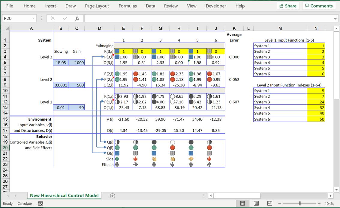
The Hierarchical Model
The display consists of three levels of control systems (Levels 1,
2 and 3) with six control systems (numbered 1-6) at each level. Each control
system is made up of three components: a reference signal, R, a perceptual
signal, P, and an output signal, O. Each of these signals is identified (in
parentheses) by its level in the
hierarchy (the first number in the parentheses) and its system number at that
level is indexed (by i, which goes from 1 to 6). So, the system at the top left
of the hierarchy is system 3,1 and the signals in that system are identified as
R(3,1), P(3,1) and O(3,1); the system at the bottom right of the hierarchy is
system 1,6 and the signals in that system are identified as R(1,6), P(1,6) and
O(1,6), etc.
This hierarchy of control systems operates in an environment
consisting of 6 physical variables, v(i), that directly affect the inputs to
the hierarchy (the Level 1 perceptual inputs), and six other physical
variables, D(i), that indirectly affect each of the corresponding v(i).
Individual Control Units
Now let’s take a closer look at an individual control system. The diagram below is of system 1,1 (the first system on the left at Level 1):
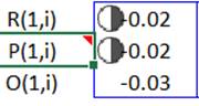
The reference signal cell, R(1,1), contains an equation that computes is the sum of the appropriate outputs coming from control systems at the next level up – Level 2 in this case. This is true for the reference signals for systems at Levels 1 and 2. The references for the systems at Level 3 – the top-level systems – can be input by the user (you); that’s why the cells containing these references are shaded yellow. These references should be set only to 1 or 0 because the perceptions controlled by these systems are logical variables so that a reference of 1 specifies that the perception be “true” and a reference of zero specifies that the perception be “false”.
The perceptual signal cell, P(1,1), contains an equation that defines the perceptual function. This is a mathematical equation that determines the aspect of the environment – the v(i)s – that is perceived and controlled by the control system. The nature of the perceptual function is the same for all systems at the same level and, therefore, determines the type of perceptual variable controlled by the systems at a particular level. The equation that defines the perceptual variables at a particular level can be seen by holding the cursor over the red triangle in the cell labeled P(). What you will see is that the systems at Level 1 control perceptions that are proportional to the magnitude of the environmental variables that are inputs to these systems, what Powers calls intensity perceptions; the systems at Level 2 control perceptions that are linear functions of the intensity perceptions that are inputs to these systems from Level 1, what Powers calls sensation perceptions; and the systems at Level 3 control perceptions that are logical function of the sensation perceptions that are inputs to these systems from Level 2, what Powers calls relationship perceptions.
The output cell , O(1,1), produces an output signal based on the difference between perception, P(1,1) and reference, R(1,1). The form of the output function is the same for all systems at all levels of the hierarchy; the general form is:
O = O + S * (G*(R – P) – O)
This is an equation for a “leaky” integrator where S is a slowing factor that determine the rate of increase in output over time and G is the gain of the control system, which determines how much output the system produces per unit error (R – P). The values of S and G are showing in the column labeled Slowing and Gain, respectively. The values of S and G are different for systems at each level. These values are currently set so that all systems are dynamically stable.
The symbols next to the reference and perceptual signals at each level of the hierarchy represent the phenomenological experience of the numerical values of these signals; that is, they represent what the numerical value of perceptual signal “looks like”. A different type of symbol is used to represent the different type of perceptions that are controlled at each level of the hierarchy. So, for example, the different levels of fill of the circles representing the intensities at Level 1 could be thought of as the different feelings for force being exerted be the muscles attached to different joints.
Controlled Variables
The hierarchy of control systems exists to control variable aspects of the system’s environment. The aspects of the environment that the system controls are called controlled variables. These variables correspond to the perceptual variables that are being controlled by the hierarchy of control systems. This is shown in the section of the spreadsheet labelled “Behavior”. The behaviors labeled Q(i) are controlled variables that correspond to the perceptual variables controlled by the hierarchy of control systems. The other behaviors shown in this section are side effects of controlling the Q(i). The Q(i) are arranged in rows that correspond (in reverse order, per the arrows) to rows of perceptions – P(1,i), P(2,i) and P(3,i) – controlled by the hierarchy. The Q(i) are not indexed by levels because an observer would not see these variables in terms of different levels. The different Q(i) would simply be seen by an observer as different variables in the environment of the system that the system is controlling. If, for example, the system is a person then an observer might see that the person is controlling a particular relationship between two different sensations – keeping, for example, the pitch of the notes they are singing a third below the note being sung by the nearby soprano.
The variables below those labeled Q(i) are labeled “Side Effects” because they represent other variables that an observer might see as what the system is doing -- variables that the system might be controlling. These other percepts are actually side effects of the system’s controlling; they are perceptual aspects of the environment that are affected by the system’s outputs but not controlled by the system. An example of such a side effect might be knocking over a cup while reaching for a pitcher of water; the perception of the cup being knocked over is a side-effect of the output (reaching) that is part of the process of controlling for grasping the pitcher. It’s not always easy to tell the difference between controlled variables and side-effects of the process of controlling those variables. Indeed, one of the main goals of research aimed at understanding the behavior of living control systems is to determine which variables they are controlling and which they are not controlling. Methods for doing this kind of research are described in my book The Study of Living Control Systems.
It is possible to change the variables that are controlled by the hierarchy of controls systems. This is done using the matrices on the right side of the display, as shown below:
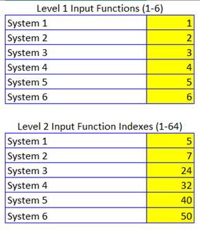
These two matrices allow you to change the perceptual variables controlled by the systems at Level 1 and Level 2 of the spreadsheet model. This is done by entering new values into the yellow highlighted cells of each matrix. The new values must be in the range shown at the top of each matrix; only integers from 1 and 6 for the Level 1 perceptions and integers from 1-64 for the Level 2 perceptions. These new values change the characteristic of a perceptual function but not its type. For example, the Level 1 perceptual functions are always intensity type perceptions defined by the function:
P (1,i) = ki * v(i)
Changing one of the values in the Level 1 matrix simply changes which one of the physical variables, v(i), is transduced into the neural perceptual signal, P(1,i). So, putting a 5 as the entry for the input function for System 1 from P (1,1) = k1 * v(1) to P (1,1) = k1 * v(5). Similarly, the Level 2 perceptual functions are always sensation type perceptions defined by the function:
P (2,i) = k1(i) * P(1,1)+ k2(i) * P(1,2) + k6(i)* P(1,6)
Changing one of the values in the Level 2 matrix changes the weights -- k1(i), k2(i) … k6(i) – of the perceptual function. For example , the “5” for Level 2, system 1, sets the weights for k1(1) thru k1(6) to 1,1,1,0,1,1. If the “5” were changed to “10” the weights would become 1,1,0,1,1,0. The system would still be controlling a sensation perception inasmuch as a linear combination of several intensities defines this type of perception. But the characteristic of this sensation perception would be different since it is now made up of a combination of a different set of intensities.
Running the Model
The hierarchical control model is designed to do what living organisms do: control perceptual aspects of a continuously changing environment. In the model, continuous changes in the environment are produced by random variations in the disturbances, D(i), over time. These random changes in D(i) are produced by running the model, which involves iteratively recalculating the spreadsheet. Running the model is, therefore, done by clicking on “Calculate” in the lower left corner of the spreadsheet window or, better, by simply pressing the F9 function key (if you are using Excel on a PC; press the “Command” and “=” keys simultaneously if you are using Excel on a Mac). When you do this the spreadsheet will instantly iterate through 10 recalculations of the spreadsheet, which will result in all disturbances having varied through 10 samples of a different low pass filtered random waveform. Continuously pressing F9 (or “Calculate) results in continuously varying D(i).
The performance of the model (in terms of how well it is controlling the controlled variables, Q(i), can be seen by monitoring the values in the “Average Error” column, which shows the average absolute deviation of perceptions from references at each level of the hierarchy. The closer these numbers are to 0.0 the better the control of the variables controlled at each level.
Experimenting with the Model
You can use the model to do many different experiments to see what kinds of things affect the ability of a hierarchical control system to control. For example, you can change the Gain and/or Slowing values to see how this affects performance. You can also see how changes in the references for the highest order variables – changing the R(3,i) values from 1 to 0 or vice versa – affects the performance of the model. You can also see how changes in the Level 1 and Level 2 Input (perceptual) functions affect performance.
I recommend doing these experiments in a copy of the Excel file that contains the model. That’s because the downloaded file automatically saves when the file is closed. This could be a problem because experimenting with the spreadsheet can result in difficult to fix problems, which will be automatically saved if you try to go back to the original state of the file by closing and then reopening it. If you work on a copy then when things go south on the copy you can close it, delete it and start over with a new copy of the downloaded original.
You are welcome to send comments, questions or suggestions regarding this spreadsheet model to me at rsmarken@gmail.com.